Example - Human Breast Cancer 10x Visium Data
In the following, we choose the human breast cancer FFPE data from 10x Visium platform as an example to display the implementation of iIMPACT on the sequencing-based SRT data.
Load Data
The current version of iIMPACT requires three input data:
The gene expression count matrix ‘count’: \(n\) by \(p\) (\(n\) - number of spots; \(p\) - number of genes)
The location information matrix ‘loc’: \(n\) by \(2\). It includes the x and y coordinate for each sample point.
The nuclei identification information matrix ‘cell_info’: \(m\) by \(3\). It includes the x and y coordinate and the nuclei class for identified cells.
The first two data should be stored in R matrix format. For gene expression count matrix, column names should be gene names.
Files can be downloaded from ‘data’ folder on the Dropbox: https://www.dropbox.com/scl/fo/em51owbpda4id0rnnin1x/h?dl=0&rlkey=nk9kc38ghs9wdjpqno7k3e1qp
# read data
cell_info <- read.csv('data/human breast cancer FFPE data/10x_breast_cancer_ffpe_cell_info.csv')
spot_loc <- read.csv('data/human breast cancer FFPE data/10x_human_breast_cancer_ffpe_loc.csv', row.names = 1)

count <- read.csv('data/human breast cancer FFPE data/10x_human_breast_cancer_ffpe_count.csv', row.names = 1)

print(dim(count))
## [1]  2518 17943

print(dim(spot_loc))
## [1] 2518    2

print(dim(cell_info))
## [1] 156235      4
This human breast cancer FFPE data has 2,518 sample points and 17,943 genes. For the histology image, the HD staining model identified 156,235 nuclei.
Process Data
Before running iIMPACT for spatial domain identification, there are several steps to prepare the data.
Generate cell abundance data
We process the nuclei segmentation results from the HD staining model to the cell abundance data \(V\) by counting the cells with different types in each expanded area.
cell_loc <- cell_info[, c('x', 'y')]
cell_type <- cell_info$nucleus_class
V <- get.cell.abundance(cell_loc, cell_type, spot_loc, lattice = 'hexagon')
## [1] "0% has been done"
## [1] "10% has been done"
## [1] "20% has been done"
## [1] "30% has been done"
## [1] "40% has been done"
## [1] "50% has been done"
## [1] "60% has been done"
## [1] "70% has been done"
## [1] "80% has been done"
## [1] "90% has been done"
## [1] "100% has been done"

print(dim(V))
## [1] 2518    7

print(head(V))
##      stroma necrosis lymphocyte blood tumor ductal epithelium macrophage
## [1,]    105        7         28    38     9                 3          2
## [2,]     60        0         37    39     0                 0          0
## [3,]     81        6         38    20     1                 0          0
## [4,]     73        2         21    15     0                 0          0
## [5,]     63        1         63    19     0                 0          0
## [6,]     86        1         70    19     0                 0          0
For the histology image, the model identified 156,235 nuclei with 7 cell types.
The obtained cell abundance data \(V\) has dimension 2,518 by 7 (\(n\) by \(q\) matrix, \(q\) is the number of cell types).
Generate low-dimensional representation of molecular profiles
Before fitting the finite mixture model, the raw gene expression counts need to be normalized and transformed to the logarithmic scale. We select the normalized expression levels of top 2,000 highly variable genes and do the dimensionality reduction to reduce the dimension using principal component analysis (PCA). Here we set the reduced dimension to be 3.
Y <- process.gene.expression(count, n_PC = 3)

print(dim(Y))
## [1] 2518    3

print(head(Y))
##          PC1       PC2        PC3
## 1 -24.172837 -4.584487  5.5806516
## 2  12.371814 -7.119854 -1.1115033
## 3  -3.332869  8.108653  0.7678203
## 4  18.560136 -5.305400  6.4929754
## 5  19.731972  4.777125  3.9005968
## 6  15.068430  3.544484 -5.7039848
Generate neighborhood information
Instead of spot coordinates, iIMPACT requires the neighbor information of spots. We apply get.neighbor function to generate the neighbor information. Sample points for this data are located on a hexagon lattice, so each spots has 6 neighbors.
G <- get.neighbor(spot_loc, 6)
Spatial Domain Identification
Run Bayesian normal-multinomial mixture model
run.iIMPACT function requires the cell abundance data from image profile \(V\), molecular profile from SRT data \(Y\) and neighborhood information \(G\) as input. We also need to set two parameters: the number of domains (clusters) ‘n_cluster’, and the scaling parameter to control the contribution of image profile ‘w’.
After fitting the finite mixture model, a label switching step is necessary. We can specify a cell type as the reference of label switching and pass the corresponding column index in \(V\) to the function via the ‘label_switch_refer’ parameter. The default index is 1.
# set number of clusters
K <- 5

# set the scaling parameter for image profile
w <- 1/20

# run iIMPACT
result <- run.iIMPACT(V, Y, G, n_cluster = K, w)
## 10% has been done
## 20% has been done
## 30% has been done
## 40% has been done
## 50% has been done
## 60% has been done
## 70% has been done
## 80% has been done
## 90% has been done
## [1] "100% has been done"
Characterize identified spatial domains
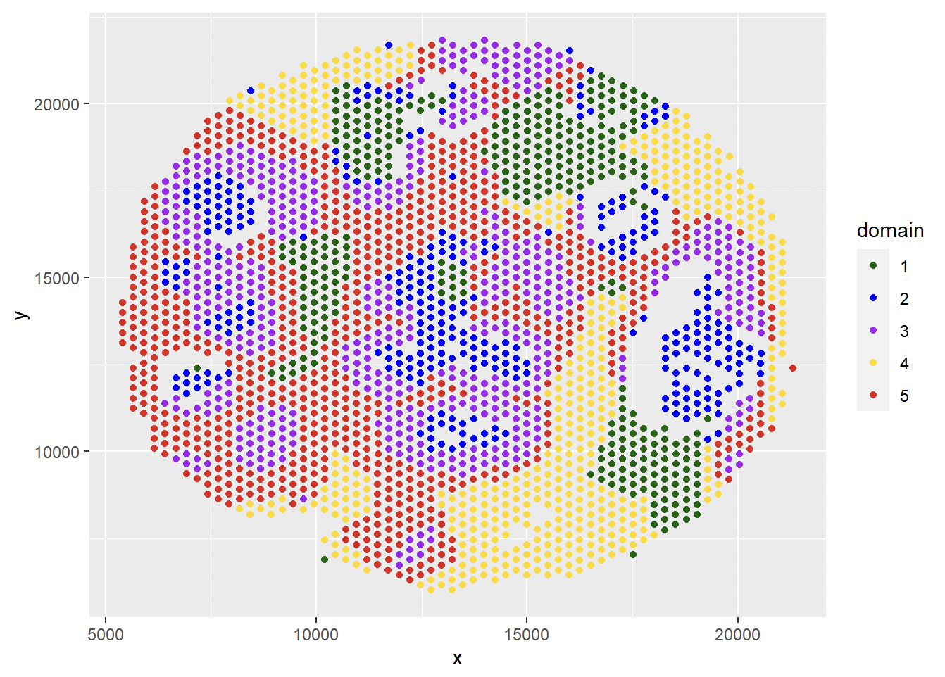
After obtaining the posterior samples of Bayesian mixture model via the run.iIMPACT function, we can obtain the spatial domain identification results via the get.spatial.domain function.
spatial_domain <- get.spatial.domain(result)

# plot results
df <- data.frame(x = spot_loc$x, y = spot_loc$y, domain = as.factor(spatial_domain))
ggplot(df, aes(x = x, y = y, color = domain)) +
  geom_point() + scale_color_manual(values=c('1' = "#006400", '2' = "#0000ff", '3' = "#A020F0", '4' = '#ffd800', '5' = '#e41a1a' ))
Get domain-level cell proportion: each row is the cell-type proportion for the corresponding domain (cluster).
domain_cell_prop <- get.domain.cell.prop(result)

print(domain_cell_prop)
##         stroma    necrosis lymphocyte      blood       tumor ductal epithelium
## [1,] 0.2407925 0.009875297 0.19702032 0.53671201 0.007796473       0.002970890
## [2,] 0.3798334 0.040353830 0.06321755 0.30010776 0.194550348       0.017041318
## [3,] 0.4022183 0.043747324 0.04294920 0.08177120 0.367408090       0.060929387
## [4,] 0.5122341 0.020637669 0.25527049 0.20140560 0.007971780       0.002090986
## [5,] 0.5443293 0.017708266 0.30624709 0.08886796 0.034487317       0.007642422
##        macrophage
## [1,] 0.0048135037
## [2,] 0.0046354940
## [3,] 0.0009506316
## [4,] 0.0001363861
## [5,] 0.0007175787
Get interactive zones: spots with high uncertainty on domain assignment.
interactive_zone <- get.interactive.zone(result)

df <- data.frame(x = spot_loc$x, y = spot_loc$y, interactive_zone = interactive_zone)
ggplot(df, aes(x = x, y = y, color = as.factor(interactive_zone))) +
  geom_point() + scale_color_manual(values=c('TRUE' = "black", 'FALSE' = "grey"))

Refine spatial domain results
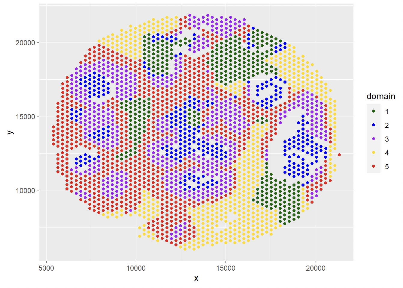
iIMPACT provides an optional refinement step for the spatial domain identification results. In this step, we need to define a parameter ‘area_unit’ as an unit of small area. For an area with the number of spots is less or equal to the ‘area_unit’, if all neighbors of this area belong to a same cluster, the clustering result of this small area will be relabeled to the same domain of its neighboring area.
spatial_domain_refined <- refine.cluster(G, spatial_domain, area_unit = 3)

# plot results
df <- data.frame(x = spot_loc$x, y = spot_loc$y, domain = spatial_domain_refined)
ggplot(df, aes(x = x, y = y, color = as.factor(domain))) +
  geom_point() + scale_color_manual(values=c('1' = "#006400", '2' = "#0000ff", '3' = "#A020F0", '4' = '#ffd800', '5' = '#e41a1a' ))
Domain-specific Spatially Variable Gene Detection
The second step of iIMPACT is to detect domain-specific SV genes based on the domains identified by the previous step via a negative binomial regression model.
Before fitting the regression model, we need to filter out genes with a high proportion of zero counts. filter.count function takes count matrix as input and can output genes (columns) with non-zero entries equal or greater than ‘min_percentage’.
count_f <- filter.count(count, min_percentage = 0.3)
We also need the estimated size factor in the regression model. get.size.factor function can estimate size factor through different methods. Here we apply total sum scaling (tss) method by setting the parameter ‘norm_method’ as ‘tss’.
size_factor <- get.size.factor(count_f, 'tss')
In the second stage of iIMPACT, a negative binomial regression model is fitted for a pre-specified spatial domain, and then domain-specific spatially variable genes can be defined via the output p-values. detect.domainSVG takes the filtered count matrix, spatial domain assignment results from the previous step, target domain index, and estimated size factor as input, and outputs the estimated coefficients for domain assignment covariate and corresponding p-values for all genes.
# set the domain for domain-specific spatially variable genes
domain_index <- 1

re <- detect.domainSVG(count_f, spatial_domain_refined, domain_index, size_factor)
# [1] "0% has been done"
## [1] "10% has been done"
## [1] "20% has been done"
## [1] "30% has been done"
## [1] "40% has been done"
## [1] "50% has been done"
## [1] "60% has been done"
## [1] "70% has been done"
## [1] "80% has been done"
## [1] "90% has been done"
## [1] "100% has been done"

print(re[1:10, ])
##       gene       beta      p_value adjusted_p_value
## 1    NOC2L -0.1831442 5.306479e-02     8.549866e-02
## 2     HES4 -0.2014012 9.506305e-03     1.870248e-02
## 3    ISG15 -0.3104067 2.107101e-09     1.177261e-08
## 4     AGRN -0.4901692 1.876475e-23     3.630437e-22
## 5     SDF4  0.1109305 6.393015e-04     1.596662e-03
## 6  B3GALT6  0.1375232 7.804545e-02     1.195188e-01
## 7   UBE2J2 -0.1196468 1.065454e-01     1.571002e-01
## 8    ACAP3 -0.2338464 1.438486e-03     3.395794e-03
## 9   INTS11 -0.1668425 2.379041e-03     5.347124e-03
## 10    CPTP -0.2228142 2.216970e-02     3.926804e-02